THE EXPANDING AND DISPERSING SAN FRANCISCO BAY AREA

by Wendell Cox 11/01/2019

This decade has witnessed an unprecedented expansion of the Greater San Francisco Bay Area (the San Jose-San Francisco combined statistical area or CSA), with the addition of three Central Valley metropolitan areas, Stockton, Modesto and Merced. Over the same period, there has been both a drop in the population growth rate and a shift of growth to the Central Valley exurban metropolitan areas. This expansion was partly justified by the increase in “extreme commutes” – one way work trips of 60 minutes or more.This increased the Bay Area’s already abundant land supply, particularly with the addition of Modesto and Merced. The Central Valley Exurbs added a plain nearly 100 miles north to south and more than 40 miles east to west.

It is notable that the Coast Mountain range did not stop the urban expansion of the Bay Area. Now, nearly 1.6 million Bay Area CSA residents live in the Central Valley exurbs (Figure 1). Much of the growth has to do with the better housing affordability there.

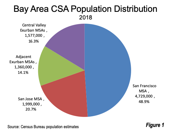
The Bay Area CSA is the broadest definition of the regional labor market, as defined by the White House Office of Management and Budget, using American Community Survey commuting data. It includes the San Francisco metropolitan area (San Francisco, Alameda, San Mateo, Contra Costa, and Marin counties), the San Jose metropolitan area (Santa Clara and San Benito counties), the Santa Rosa metropolitan area (Sonoma County), the Vallejo metropolitan area (Solano County), the Napa metropolitan area (Napa County), the Santa Cruz metropolitan area (Santa Cruz County), the Stockton metropolitan area (San Joaquin County) and the Modesto metropolitan area (Stanislaus) and the Merced metropolitan area (Merced County). The latter shares its southern border with the Fresno CSA.

Population Growth Dropping and Shifting from the Center

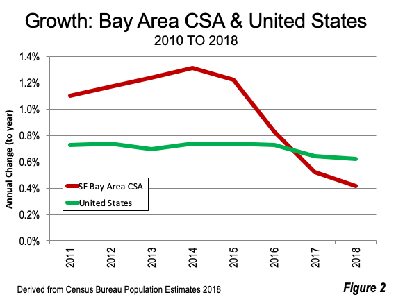
Earlier in the decade (2010 – 2015), propelled by the tech boom, the Bay Area CSA experienced strong growth, adding 1.2% annually to its population. This is more than 50% above the national population growth rate of 0.7% (Figure 2). The last three years, however (2015 – 2018) the population growth rate fell to 0.6%, half that of the 2010 – 2015 rate, well below the national rate. Virtually all of the declining growth rate is attributable to the San Francisco and San Jose metropolitan areas, along with the adjacent exurban metropolitan areas (Santa Rosa, Vallejo, Napa and Santa Cruz).

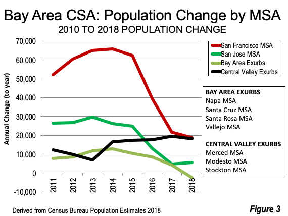
The San Francisco metropolitan area added fewer than 19,000 new residents in 2017 – 2018, a full two thirds below its 60,000 average increase for 2010 – 2015. The San Jose metropolitan area added fewer than 6000 new residents in 2017 – 2018, down approximately 80% from its annual growth of more than 25,000 in 2010 to 2015. The adjacent exurbs, which had added an average of 10,000 residents from 2010 – 2015 saw their growth collapse to a 2000 loss in 2018.This is all the more remarkable in the face of what has been a remarkable economic boom.

Only the Central Valley metropolitan areas sustained their growth, increasing from an annual average of nearly 13,000 in 2010 – 2015 to nearly 18,000 in 2015 – 2018 (Figure 3).

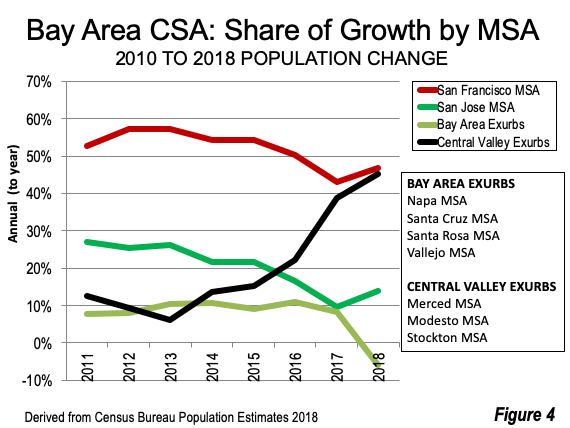
The shift of growth to the Central Valley is illustrated by the tripling of its share of Bay Area CSA growth from 11% in 2010 – 2015 to 35% from 2015 to 2018. The San Francisco metropolitan area fell from 55% of the growth in the first five years to 46% in the last three. The San Jose metropolitan area growth has been nearly halved from 24% to 13%. The adjacent exurbs accounted for 9% of growth in 2010 – 2015, dropping by more than half to 4% between 2015 and 2018 and losing population in 2017 - 2018 (Figure 4).

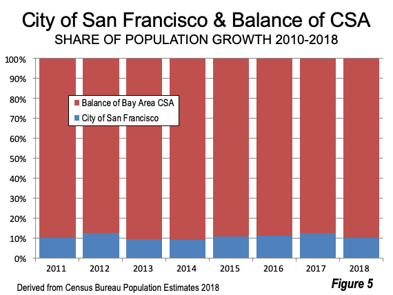
Even so, the city of San Francisco, which accounts for much of the urban core population, has maintained its growth share, having captured 10.6% of the 2010 – 2015 growth and a slightly larger 11.4% in 2015 – 2018 (Figure 5).

Declining Natural Increase Rate

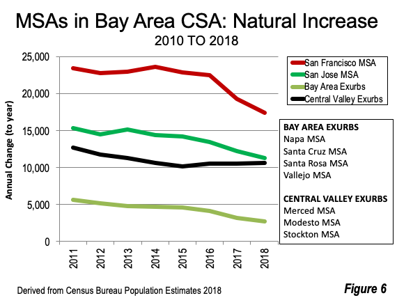
The Bay Area’s annual natural increase in population has been declining. This measure, measured by births minus deaths, dropped from 57,000 in 2010 – 2011 to 42,000 in 2017 – 2018, an overall decline of 26%. The decline was similar in the San Francisco and San Jose metropolitan areas. The largest decline was in the adjacent exurbs, where the natural increase rate declined by more than one half, from 5600 to 2700. The smallest decline was in the Central Valley exurbs, at 17% (Figure 6). The total natural increase was nearly 410,000.

The natural population increase is declining across the nation, due to falling fertility rates. The recent collapse in the Bay Area CSA in domestic outmigration is also a factor. IRS data shows that California’s net domestic outmigration tends to be strongest among households from 26 to 44 years old, ages that produce most of the children. The lowest outmigration rate is among those aged 65 and over.

Meanwhile, Marin County has the oldest median age in the CSA, at 47.2 years. More than nine years older than the national median (38.4). The youngest ages are in the Central Valley exurbs. Merced County has a median age of 32.1, while San Joaquin and Stanislaus counties are at 34.5.

Domestic Migration Collapses

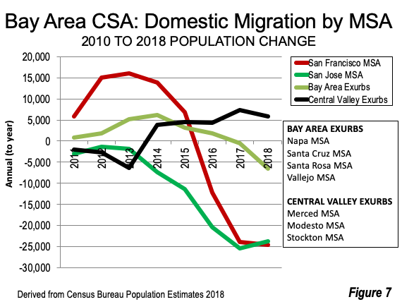
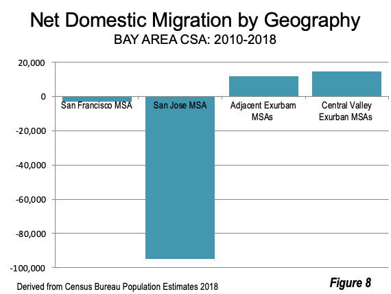
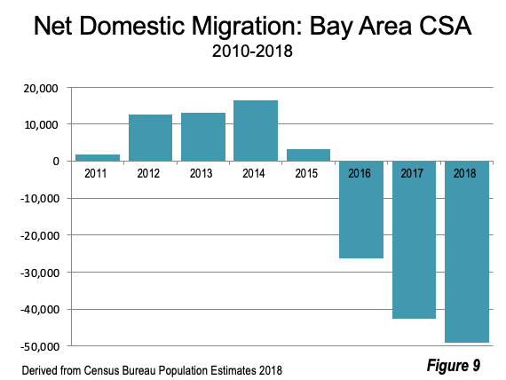
The Bay Area CSA gained an average of 9000 domestic migrants in 2010 – 2015. However, domestic migration collapsed to an annual net loss of 39,000 in 2015 – 2018, reaching a loss of nearly 50,000 in 2017 – 2018 (Figure 7). Net domestic migration dropped strongly in both the San Francisco and San Jose metropolitan areas. The Bay Area CSA net domestic migration loss in 2010 – 2018 was 71,000.

The decline in net domestic migration was less severe in the adjacent exurbs. The Central Valley exurbs experienced positive domestic migration, reversing the early losses that had been precipitated by the devastating effects of the Great Recession (Figure 7).

The overall 2000 – 2018 net domestic migration by metropolitan area is shown in Figure 8. The overall decline in Bay Area CSA net domestic migration is illustrated in Figure 9.

International Migration

Net international migration has been more steady, ranging from approximately 40,000 to 60,000 per year, with similar fluctuations throughout the CSA. Net international migration was nearly 390,000 from 2010-2018.

Growth Increasing Only in the Central Valley Exurbs

To summarize, the 2010 – 2008 components of population change in the Bay Area CSA are indicated in Figure 10.

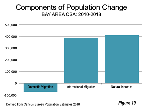
The Bay Area CSA has seen a significant reduction in its pattern of growth as the decade has proceeded. The result is that growth has been largely stunted in the San Francisco, San Jose and adjacent metropolitan areas, with growth increasing only in the Central Valley exurbs. The Bay Area may remain the tech capital of the world, people are moving away, despite the continued economic growth.

Photograph: Central Valley Bay Area Exurbs: From the Stockton metropolitan area, looking south toward the Modesto and Merced metropolitan areas (by author).

Wendell Cox is principal of Demographia, an international public policy and demographics firm. He is a Senior Fellow of the Center for Opportunity Urbanism (US), Senior Fellow for Housing Affordability and Municipal Policy for the Frontier Centre for Public Policy (Canada), and a member of the Board of Advisors of the Center for Demographics and Policy at Chapman University (California). He is co-author of the "Demographia International Housing Affordability Survey" and author of "Demographia World Urban Areas" and "War on the Dream: How Anti-Sprawl Policy Threatens the Quality of Life." He was appointed by Mayor Tom Bradley to three terms on the Los Angeles County Transportation Commission, where he served with the leading city and county leadership as the only non-elected member. Speaker of the House of Representatives appointed him to the Amtrak Reform Council. He served as a visiting professor at the Conservatoire National des Arts et Metiers, a national university in Paris.

DISPERSED AMERICAN URBAN FORM YIELDS QUICK WORK TRIPS

by Wendell Cox 08/09/2018

Planners and journalists are often uneasy about suburban development, wondering how people will get to work in the center from more distant locations. They needn’t worry. Only a relatively small percentage of people work in the center (generally less than 10 percent). Indeed the residential employment dispersion in American metropolitan areas has been a major factor in keeping work trip travel times among the shortest in the world.

In a ground breaking 2007 research paper, economists Bumsoo Lee and Peter Gordon cited William T. Bogart, now president of Maryville College (Tennessee), to dismiss the pervasive idea in planning, media and academic circles that American metropolitan areas (cities in their economic or functional form) still exhibit the monocentric form that ceased to be long ago.

“A fundamental misunderstanding of how metropolitan areas work has hampered the current debate on the causes and consequences of urban sprawl. This misunderstanding is analogous to the pre-Copernican fallacy that the earth is the center of the universe, and everything revolves around the earth. In the discussion of urban sprawl, the downtown or central city takes the place of the earth in the Ptolemaic cosmology, and the rest of the metropolitan area is defined only in relation to the downtown.”

In their research, Lee and Gordon showed that as early as 2000, no major metropolitan area (over 1 million population) in the United States had a monocentric employment pattern. Indeed, they showed that US metropolitan areas were already more polycentric than monocentric. That includes New York, where more than 75 percent of employment was outside the monocentric core (the central business district or CBD) and other major subcenters.

But the real momentum is beyond polycentrism, to dispersal outside of even suburban business centers. (Figure 1). Earlier, Gordon and Harry Richardson showed that Los Angeles had left polycentricity behind for a dispersed urban form by 1990. Although the Lee and Gordon research has not been updated, the most recent Census Bureau County Business Patterns data shows that 94 percent of new employment has been located in two outer sectors (Later Suburbs & Exurbs) since 2000 (Figures 2 & 3).

This analysis uses the City Sector Model and American Community Survey (2012-2016) to estimate average work trip travel times for 2016 for sectors within major metropolitan areas (See Note and Figure 11). This demonstrates that across the entire US metropolitan area, average one-way work trip travel times are around 30 minutes or less.

Evenly Dispersed Residences & Employment

Jobs and resident workers are relatively balanced in US metropolitan areas. In the suburbs and exurbs, there are 0.95 jobs per resident worker, and 1.28 resident jobs per resident workers in the Urban Core (Figure 4). This figure, however, masks the distorted ratio in the Urban Core CBD, which has by far the highest employment density of any sector, nearly 20 times that of the second densest sector (Urban Core: Inner Ring) and 60 times that of the Earlier Suburbs, which have nearly five times as many jobs (Figure 6). Yet despite its extreme concentration of employment, the Urban Core: CBD still only represents less than 10 percent of overall employment.

Travel Times

This dispersion works to the advantage of commuters, whose travel times are remarkably similar throughout metropolitan areas.

Overall, suburban and exurban commuters have faster travel times (28.1 minutes) on average to work than those living (Figure 7) in the urban cores (32.7 minutes). The greatest disparities are in the largest metropolitan areas, such as in New York, Los Angeles, Chicago, and Philadelphia where urban core commuters travel for much longer to get to work, (Table). Nonetheless, in many other metropolitan areas, urban ore residents have quicker work trip travel time than those in the suburbs and exurbs. Overwhelmingly, these are where there is greater auto use (cars have quicker work trips, see below), together with low enough densities to limit traffic congestion.

The finer grained sectoral analysis shows that workers living in the Earlier Suburbs have the shortest commutes, at 27.2 minutes. Those living in the Urban Core: CBD have the second shortest travel times, at 27.4 minutes (Figure 8). Neither of these results are surprising. The Earlier suburbs are more accessible to the rest of the city, since they are closer to the four other sectors and they have the most jobs. The shorter travel times of the Urban Core: CBD make the chances of finding suitable employment that can be reached more quickly, with six times as many jobs as workers. Obviously, this cannot be replicated throughout the metropolitan area, since by definition, labor markets have about the same number of jobs and employed workers.

The longest travel time among the five sectors is in the Urban Core: Inner Ring, at 33.3 minutes. The outer two sectors, the Later Suburbs and the Exurbs have travel times of 28.5 minutes and 29.9 minutes, close to the average of 28.8 minutes. This demonstrates the effectiveness of automobile oriented residential and employment density in keeping travel times down. It is worth noting that more dense international cities, that are the most dependent on transit, tend to suffer longer commuting times, such as Hong Kong and Tokyo.

Among the largest commuting modes (excluding working at home with its commute time of zero), driving alone takes the least time, averaging 28.2 minutes for urban core residents and 26.6 minutes for suburban and exurban residents. In both cases, car pools travel about three minutes longer. Transit takes much longer, 46.4 minutes for urban core residents and 55.3 minutes for suburban and exurban residents (Figure 9). Among the five sectors, there is little difference in commuting times for those who drive along or are in car pools.

Transit travel times rise rapidly as distances increase from the CBD (Figure 10). This is to be expected, since transit systems are necessarily designed principally to serve the CBDs, where employment densities are high enough to justify frequent service, despite massive subsidies. Elsewhere in the metropolitan area, that is simply not the case, with automobiles providing access to more than 60 times as many jobs in 30 minutes as transit in the major metropolitan areas (see: “Focusing on Mobility, Not Travel Mode for Better Economic Growth”). With this kind of disparity, it is not hard to understand why automobiles dominate travel in the modern city.

Maintaining Quicker Travel Times

Yet, for decades, transit promoters have claimed that much more transit spending would reduce traffic congestion. This just has not happened. Perhaps the starkest example is Los Angeles County, which has seen driving and working at home capture 99 percent of the nearly 350,000 new daily commutes over the last decade (according to American Community Survey data), and an overall drop in transit commuting, despite a Herculean pace of new rail and busway openings. Yet, quick work trip travel times remain integral to improved economic performance. Continuing dedication and efforts to provide sufficient roadway capacity are needed to “keep the traffic moving”, perhaps with the aid of new technologies such as ride-hailing and, down the road, autonomous vehicles.

Note: The City Sector Model classifies small areas based upon their urban characteristics, with two urban core sectors (Urban Core: CBD and Urban Core: Inner Ring) having higher population densities, and greater dependence on transit, walking and cycling. The three other sectors, Earlier Suburbs, Later Suburbs and Exurbs are more automobile oriented and tend to have the suburban forms that have dominated development since World War II. City Sector Model analysis provides results that are far more accurate in measuring urban cores versus suburban and exurban development than using municipal boundaries, since the most of the core municipalities have the majority of their population in areas with suburban and exurban characteristics and none is 100 percent urban core. For example, even in the city of New York, much of Staten Island is at least as suburban as the adjacent New Jersey suburbs).

Photograph: Los Angeles Urban Area Freeway (densest large urban area in the United States), by author

AVERAGE WORK TRIIP TRAVEL TIMES: 2016
US Major Metropolitan Areas
Major Metropolitan Area	Urban Core	Suburbs & Exurbs	Entire MSA
Atlanta, GA	21.8	31.0	31.0
Austin, TX	17.1	26.6	26.4
Baltimore, MD	29.8	30.6	30.5
Birmingham, AL		26.0	26.0
Boston, MA-NH	29.8	31.1	30.6
Buffalo, NY	20.4	21.6	21.3
Charlotte, NC-SC		26.3	26.3
Chicago, IL-IN-WI	33.5	30.6	31.3
Cincinnati, OH-KY-IN	20.9	25.0	24.6
Cleveland, OH	24.0	24.8	24.6
Columbus, OH	19.0	23.7	23.5
Dallas-Fort Worth, TX	23.1	27.8	27.8
Denver, CO	22.9	27.5	27.3
Detroit,  MI	26.4	26.7	26.7
Grand Rapids, MI	19.9	22.0	21.9
Hartford, CT	22.1	24.0	23.8
Houston, TX	19.9	29.5	29.4
Indianapolis. IN	22.6	24.9	24.8
Jacksonville, FL		26.3	26.3
Kansas City, MO-KS	19.9	23.1	22.9
Las Vegas, NV	26.3	24.3	24.4
Los Angeles, CA	31.0	29.5	29.6
Louisville, KY-IN	21.6	23.9	23.7
Memphis, TN-MS-AR	19.5	24.1	24.0
Miami, FL	26.6	28.6	28.5
Milwaukee,WI	21.9	23.5	23.2
Minneapolis-St. Paul, MN-WI	22.5	25.6	25.2
Nashville, TN	14.6	27.1	27.1
New Orleans. LA	20.5	26.4	25.7
New York, NY-NJ-PA	38.9	32.6	35.9
Oklahoma City, OK	16.4	22.6	22.4
Orlando, FL		27.9	27.9
Philadelphia, PA-NJ-DE-MD	32.2	28.3	29.2
Phoenix, AZ		26.0	26.0
Pittsburgh, PA	24.7	26.9	26.5
Portland, OR-WA	24.0	26.4	26.1
Providence, RI-MA	23.4	26.3	25.6
Raleigh, NC		25.3	25.3
Richmond, VA	19.2	25.4	25.1
Riverside-San Bernardino, CA		31.8	31.8
Rochester, NY	19.7	21.4	21.2
Sacramento, CA	21.8	26.4	26.3
St. Louis,, MO-IL	23.1	25.8	25.5
Salt Lake City, UT	18.8	22.7	22.5
San Antonio, TX	17.1	25.7	25.6
San Diego, CA	22.3	25.4	25.3
San Francisco-Oakland, CA	31.7	32.4	32.2
San Jose, CA	21.1	27.3	27.3
Seattle, WA	25.4	30.2	29.6
Tampa-St. Petersburg, FL		26.7	26.7
Tucson, AZ		24.3	24.3
Virginia Beach-Norfolk, VA-NC	18.9	24.2	24.1
Washington, DC-VA-MD-WV	30.6	35.3	34.4
TOTAL	32.7	28.1	28.8
Derived from American Community Survey, 2016.

Wendell Cox is principal of Demographia, an international public policy and demographics firm. He is a Senior Fellow of the Center for Opportunity Urbanism (US), Senior Fellow for Housing Affordability and Municipal Policy for the Frontier Centre for Public Policy (Canada), and a member of the Board of Advisors of the Center for Demographics and Policy at Chapman University (California). He is co-author of the "Demographia International Housing Affordability Survey" and author of "Demographia World Urban Areas" and "War on the Dream: How Anti-Sprawl Policy Threatens the Quality of Life." He was appointed to three terms on the Los Angeles County Transportation Commission, where he served with the leading city and county leadership as the only non-elected member. He served as a visiting professor at the Conservatoire National des Arts et Metiers, a national university in Paris.

What is Middle-Income Housing Affordability?

What is Middle-Income Housing Affordability? 

by Wendell Cox

Few local or metropolitan issues receive more attention than housing affordability. This article provides a perspective on housing affordability. The focus is on the approach used by the Demographia International Housing Affordability Survey, which I co-author annually with Hugh Pavletich (of performanceurbanplanning.org). The Demographia Survey has been published for 14 years. This edition includes housing affordability data and ratings for nearly 300 cities (metropolitan areas) in nine nations (Note 1).
What is Housing Affordability?

Housing affordability is the relationship between housing costs and income. Affordability can only be evaluated if there is a comparison to income. Yet, analysts and journalists often use refer to house prices or rents or their increases without relation to incomes to describe housing affordability. Prices are not an indicator of affordability if they are not compared to incomes but have only anecdotal value. Nor are house price or rent trends an indicator of affordability without comparison to incomes.
What is Middle-Income Housing Affordability?

Middle-income housing affordability is important, because affordable access to quality housing has been pivotal to the democratization of prosperity that occurred in the last century in most high-income nations. Normally, the competitive market has provided middle-income housing without the need for subsidies.

Middle-income is different from low – income housing (also called “affordable housing” or “social housing”), which relies on public subsidies to serve the needs of households unable to afford the house prices or rents prevailing on the open market. Focusing on middle-income does not indicate a lesser interest in low-income housing, because subsidy eligibility requirements are tied to house prices. Better housing affordability translates into fewer households seeking housing subsidies through affordable housing programs (and less public expense).

There are two principal dimensions of middle-income housing affordability — between housing markets and within individual market over time.
Owned and Rented Housing Affordability

Housing affordability can be measured for both owned and rented housing. Price-to-income ratios are typical for owned housing, including the “median multiple” used in the Demographia Survey (below). Percentage of incomes spent on rents are often used to evaluate rental housing affordability.

The Importance of Middle-Income Housing Affordability

Housing is usually the largest budget item for households. The differences in housing costs between major metropolitan areas now increasingly drive differences in the costs of living. Housing costs also vary far more in their high to low range than in the other two major expenditure categories, according to the US Bureau of Economic Analysis, which are services not including rents and goods. (Figure 1).

The differences are even greater when the costs of owned housing are included, as is illustrated by the COU “movers” cost of living index. This index estimates the cost of living for a domestic migrant household moving into the housing market and captures both the differences in rental and owned housing affordability. It is estimated that in the high-cost markets, 85 percent of the higher cost of living stems from higher housing costs (Figure 2).

Middle-income housing affordability is also important to the economy. Paul Cheshire of the London School of Economics and Wouter Vermeulen of VU University wrote, “… [h]ousing being the dominant asset in most households’ portfolios, there are also repercussions on saving, investment and consumption choices.” Where housing is more affordable, households will have more discretionary income to purchase additional goods and services and to save (which generates investment). All of this can contribute to job creation and a stronger economy.

Not only do higher house prices lead to a lower standard of living, but can also increase poverty. For example, California has the highest housing cost adjusted poverty rate among the 50 states of the United States, at 20.4%. This compares to California’s 14.5% rate without adjustment for housing costs.

Owned Housing Affordability Metrics

One of the most utilized owned housing affordability metrics is the price-to-income ratio. A United Nations publication indicated:


“If there is a single indicator that conveys the greatest amount of information on the overall performance of housing markets, it is the house price-to-income ratio. It is obviously a key measure of housing affordability. When housing prices are high relative to incomes, other things being equal, a smaller fraction of the population will be able to purchase housing.”

The Demographia International Housing Affordability Survey uses the median multiple (median house price divided by median household income). The evaluation criteria is in Figure 3.

The Geography of Housing Affordability

Demographia evaluates housing affordability between housing markets: Housing markets are coterminous with labor markets (metropolitan areas). Within housing markets, there will typically be a large urban area, which is defined an expanse of contiguous built-up land (see Demographia World Urban Areas). The area beyond the urban periphery is defined as the urban fringe, which is generally the land between the principal urban area and the boundaries of the metropolitan area. Typically, the urban fringe contains virtually all of the greenfield (undeveloped) land that can be used for new housing. Much of the growth of urban areas that has occurred since World War II in Australia, Canada, New Zealand, and the United States has been in detached housing tracts in greenfield areas.

Thus, for example, the New York housing market includes the entire New York metropolitan area, which stretches from Montauk Point on Long Island (east) to Pike County, Pennsylvania (west) to Ocean County, New Jersey (south) and to Dutchess County (north). The city of New York and other municipalities are only parts of the New York housing market.

Housing affordability may also be evaluated within a housing market. For example, the housing affordability in Brooklyn can be compared to that of White Plains. Or, housing affordability can be compared between more local neighborhoods, like Rainier Valley and Ballard in Seattle. Demographia evaluates housing affordability only at the housing market level and thus does not evaluate housing affordability between areas within housing markets.

The Time Dimension of Housing Affordability

The other important housing affordability comparison is historical, or over time. Thus, housing affordability may be compared for the same or multiple housing markets between 2000 and 2017.
The Need for Clarity

As many cities evaluated by Demographia suffer severe housing affordability, evaluations need to be conducted with sufficient clarity. Serious housing affordability evaluation requires comparison that includes incomes, as well as comparisons between housing markets and over time. In fact, much of the nation remains affordable by historic standards — severe unaffordability is limited to a minority of markets. The public is misled by analyses that fail to include both prices and incomes (See related article: “Housing Affordability from Vancouver to Sydney and Toronto: Time to Do What Works“).

Note 1: Metropolitan areas are “economic cities,” generally not related to the physical jurisdictions of cities as local government authorities, which may be larger or smaller than metropolitan areas.

Note 2: Parts of this article are adapted from published materials I have authored or co-authored.


Wendell Cox is principal of Demographia, an international public policy and demographics firm. He is a Senior Fellow of the Center for Opportunity Urbanism (US), Senior Fellow for Housing Affordability and Municipal Policy for the Frontier Centre for Public Policy (Canada), and a member of the Board of Advisors of the Center for Demographics and Policy at Chapman University (California). He is co-author of the “Demographia International Housing Affordability Survey” and author of “Demographia World Urban Areas” and “War on the Dream: How Anti-Sprawl Policy Threatens the Quality of Life.” He was appointed to three terms on the Los Angeles County Transportation Commission, where he served with the leading city and county leadership as the only non-elected member. He served as a visiting professor at the Conservatoire National des Arts et Metiers, a national university in Paris